Omitted Variable Bias And How To Deal With It
In causal inference, bias is extremely problematic because it makes inference not valid. Bias generally means that an estimator will not deliver the estimate of the true effect, on average.
This is why, in general, we prefer estimators that are unbiased, at the cost of a higher variance, i.e. more noise. Does it mean that every biased estimator is useless? Actually no. Sometimes, with domain knowledge, we can still draw causal conclusions even with a biased estimator.
In this post, we are going to review a specific but frequent source of bias, omitted variable bias (OVB). We are going to explore the causes of the bias and leverage these insights to make causal statements, despite the bias.
Theory
Suppose we are interested in the effect of a variable $D$ on a variable $y$. However, there is a third variable $Z$ that we do not observe and that is correlated with both $D$ and $Y$. Assume the data generating process can be represented with the following Directed Acyclic Graph (DAG). If you are not familiar with DAGs, I have written a short introduction here.
flowchart LR
classDef included fill:#DCDCDC,stroke:#000000,stroke-width:2px;
classDef excluded fill:#ffffff,stroke:#000000,stroke-width:2px;
classDef unobserved fill:#ffffff,stroke:#000000,stroke-width:2px,stroke-dasharray: 5 5;

D((D))
Z((Z))
Y((Y))

D --> Y
Z --> D
Z --> Y

class D,Y excluded;
class Z unobserved;
Since there is a backdoor path from $D$ to $y$ passing through $Z$, we need to condition our analysis on $Z$ in order to recover the causal effect of $D$ on $y$. If we could observe $Z$, we would run a linear regression of $y$ on $D$ and $Z$ to estimate the following model:
$$ y = \alpha D + \gamma Z + \varepsilon $$
where $\alpha$ is the effect of interest. This regression is usually referred to as the long regression since it includes all variables of the model.
However, since we do not observe $Z$, we have to estimate the following model:
$$ y = \alpha D + u $$
The corresponding regression is usually referred to as the short regression since it does not include all the variables of the model
What is the consequence of estimating the short regression when the true model is the long one?
In that case, the OLS estimator of $\alpha$ is
$$ \begin{align} \hat \alpha &= \frac{Cov(D, y)}{Var(D)} = \newline &= \frac{Cov(D, \alpha D + \gamma Z + \varepsilon)}{Var(D)} = \newline &= \frac{Cov(D, \alpha D)}{Var(D)} + \frac{Cov(D, \gamma Z)}{Var(D)} + \frac{Cov(D, \varepsilon)}{Var(D)} = \newline &= \alpha + \underbrace{ \gamma \frac{Cov(D, Z)}{Var(D)} }_{\text{omitted variable bias}} \end{align} $$
Therefore, we can write the omitted variable bias as
$$ \text{OVB} = \gamma \delta \qquad \text{ where } \qquad \delta := \frac{Cov(D, Z)}{Var(D)} $$
The beauty of this formula is its interpretability: the omitted variable bias consists in just two components, both extremely easy to interpret.
- $\gamma$: the effect of $Z$ on $y$
- $\delta$: the effect of $D$ on $Z$
Additional Controls
What happens if we had additional control variables in the regression? For example, assume that besides the variable of interest $D$, we also observe a vector of other variables $X$ so that the long regression is
$$ y = \alpha D + \beta X + \gamma Z + \varepsilon $$
Thanks to the Frisch-Waugh-Lowell theorem, we can simply partial-out $X$ and express the omitted variable bias in terms of $D$ and $Z$.
$$ \text{OVB} = \gamma \times \frac{Cov(D^{\perp X}, Z^{\perp X})}{Var(D^{\perp X})} $$
where $D^{\perp X}$ are the residuals from regressing $D$ on $X$ and $Z^{\perp X}$ are the residuals from regressing $Z$ on $X$. If you are not familiar with Frisch-Waugh-Lowell theorem, I have written a short note here.
Chernozhukov, Cinelli, Newey, Sharma, Syrgkanis (2022) further generalize to analysis the the setting in which the control variables $X$ and the unobserved variables $Z$ enter the long model with a general functional form $f$
$$ y = \alpha D + f(Z, X) + \varepsilon $$
You can find more details in their paper, but the underlying idea remains the same.
Example
Suppose we were a researcher interested in the relationship between education and wages. Does investing in education pay off in terms of future wages? Suppose we had data on wages for people with different years of education. Why not looking at the correlation between years of education and wages?
The problem is that there might be many unobserved variables that are correlated with both education and wages. For simplicity, let’s concentrate on ability. People of higher ability might decide to invest more in education just because they are better in school and they get more opportunities. On the other hand, they might also get higher wages afterwards, purely because of their innate ability.
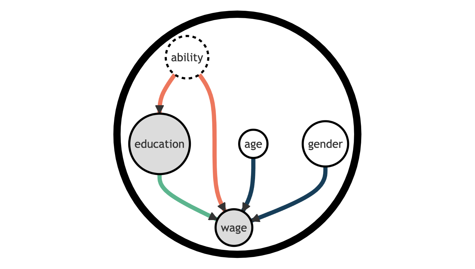
We can represent the data generating process with the following Directed Acyclic Graph (DAG).
flowchart TD
classDef included fill:#DCDCDC,stroke:#000000,stroke-width:2px;
classDef excluded fill:#ffffff,stroke:#000000,stroke-width:2px;
classDef unobserved fill:#ffffff,stroke:#000000,stroke-width:2px,stroke-dasharray: 5 5;

D((education))
Z((ability))
Y((wage))
X1((age))
X2((gender))

D --> Y
Z --> D
Z --> Y
X1 --> Y
X2 --> Y

class D,Y included;
class X1,X2 excluded;
class Z unobserved;
Let’s load and inspect the data. I import the data generating process from src.dgp and some plotting functions and libraries from src.utils.
%matplotlib inline
%config InlineBackend.figure_format = 'retina'
from src.utils import *
from src.dgp import dgp_educ_wages

df = dgp_educ_wages().generate_data(N=50)
df.head()
| age | gender | education | wage | |
|---|---|---|---|---|
| 0 | 62 | male | 6.0 | 3800.0 |
| 1 | 44 | male | 8.0 | 4500.0 |
| 2 | 63 | male | 8.0 | 4700.0 |
| 3 | 33 | male | 7.0 | 3500.0 |
| 4 | 57 | female | 6.0 | 4000.0 |
We have information on 300 individuals, for which we observe their age, their gender, the years of education, and the current monthly wage.
Suppose we were directly regressing wage on education.
short_model = smf.ols('wage ~ education + gender + age', df).fit()
short_model.summary().tables[1]
| coef | std err | t | P>|t| | [0.025 | 0.975] | |
|---|---|---|---|---|---|---|
| Intercept | 2657.8864 | 444.996 | 5.973 | 0.000 | 1762.155 | 3553.618 |
| gender[T.male] | 335.1075 | 132.685 | 2.526 | 0.015 | 68.027 | 602.188 |
| education | 95.9437 | 38.752 | 2.476 | 0.017 | 17.940 | 173.948 |
| age | 12.3120 | 6.110 | 2.015 | 0.050 | 0.013 | 24.611 |
The coefficient of education is positive and significant. However, we know there might be an omitted variable bias, because we do not observe ability. In terms of DAGs, there is a backdoor path from education to wage passing through ability that is not blocked and therefore biases our estimate.
flowchart TD
classDef included fill:#DCDCDC,stroke:#000000,stroke-width:2px;
classDef excluded fill:#ffffff,stroke:#000000,stroke-width:2px;
classDef unobserved fill:#ffffff,stroke:#000000,stroke-width:2px,stroke-dasharray: 5 5;

D((education))
Z((ability))
Y((wage))
X1((age))
X2((gender))

D --> Y
Z --> D
Z --> Y
X1 --> Y
X2 --> Y

class D,Y included;
class X1,X2 excluded;
class Z unobserved;

linkStyle 0 stroke:#00ff00,stroke-width:4px;
linkStyle 1,2 stroke:#ff0000,stroke-width:4px;
Does it mean that all our analysis is garbage? Can we still draw some causal conclusion from the regression results?
Direction of the Bias
If we knew the signs of $\gamma$ and $\delta$, we could infer the sign of the bias, since it’s the product of the two signs.
$$ \text{OVB} = \gamma \delta \qquad \text{ where } \qquad \gamma := \frac{Cov(Z, y)}{Var(Z)}, \quad \delta := \frac{Cov(D, Z)}{Var(D)} $$
which in our example is
$$ \text{OVB} = \gamma \delta \qquad \text{ where } \qquad \gamma := \frac{Cov(\text{ability}, \text{wage})}{Var(\text{ability})}, \quad \delta := \frac{Cov(\text{education}, \text{ability})}{Var(\text{education})} $$
Let’s analyze the two correlations separately:
- The correlation between
abilityandwageis most likely positive - The correlation between
abilityandeducationis most likely positive
Therefore, the bias is most likely positive. From this, we can conclude that our estimate from the regression on wage on education is most likely an overestimate of the true effect, which is most likely smaller.
This might seem like a small insight, but it’s actually huge. Now we can say with confidence that one year of education increases wages by at most 95 dollars per month, which is a much more informative statement than just saying that the estimate is biased.
In general, we can summarize the different possible effects of the bias in a 2-by-2 table.

Further Sensitivity Analysis
Can we say more about the omitted variable bias without making strong assumptions?
The answer is yes! In particular, we can ask ourselves: how strong should the partial correlations $\gamma$ and $\delta$ be in order to overturn our conclusion?
In our example, we found a positive correlation between education and wages in the data. However, we know that we are omitting ability in the regression. The question is: how strong should the correlation between ability and wage, $\gamma$, and between ability and education, $\delta$, be in order to make the effect not significant or even negative?
Cinelli and Hazlett (2020) show that we can transform this question in terms of residual variation explained, i.e. the coefficient of determination, $R^2$. The advantage of this approach is interpretability. It is much easier to make a guess about the percentage of variance explained than to make a guess about the magnitude of a conditional correlation.
The authors wrote a companion package sensemakr to conduct the sensitivity analysis. You can find a detailed description of the package here.
We will now use the Sensemakr function. The main arguments of the Sensemakr function are:
model: the regression model we want to analyzetreatment: the feature/covariate of interest, in our caseeducation
The question we will try to answer is the following:
How much of the residual variation in
education(x axis) andwage(y axis) doesabilityneed to explain in order for the effect ofeducationonwagesto change sign?
import sensemakr

sensitivity = sensemakr.Sensemakr(model = short_model, treatment = "education")
sensitivity.plot()
plt.xlabel("Partial $R^2$ of ability with education");
plt.ylabel("Partial $R^2$ of ability with wage");
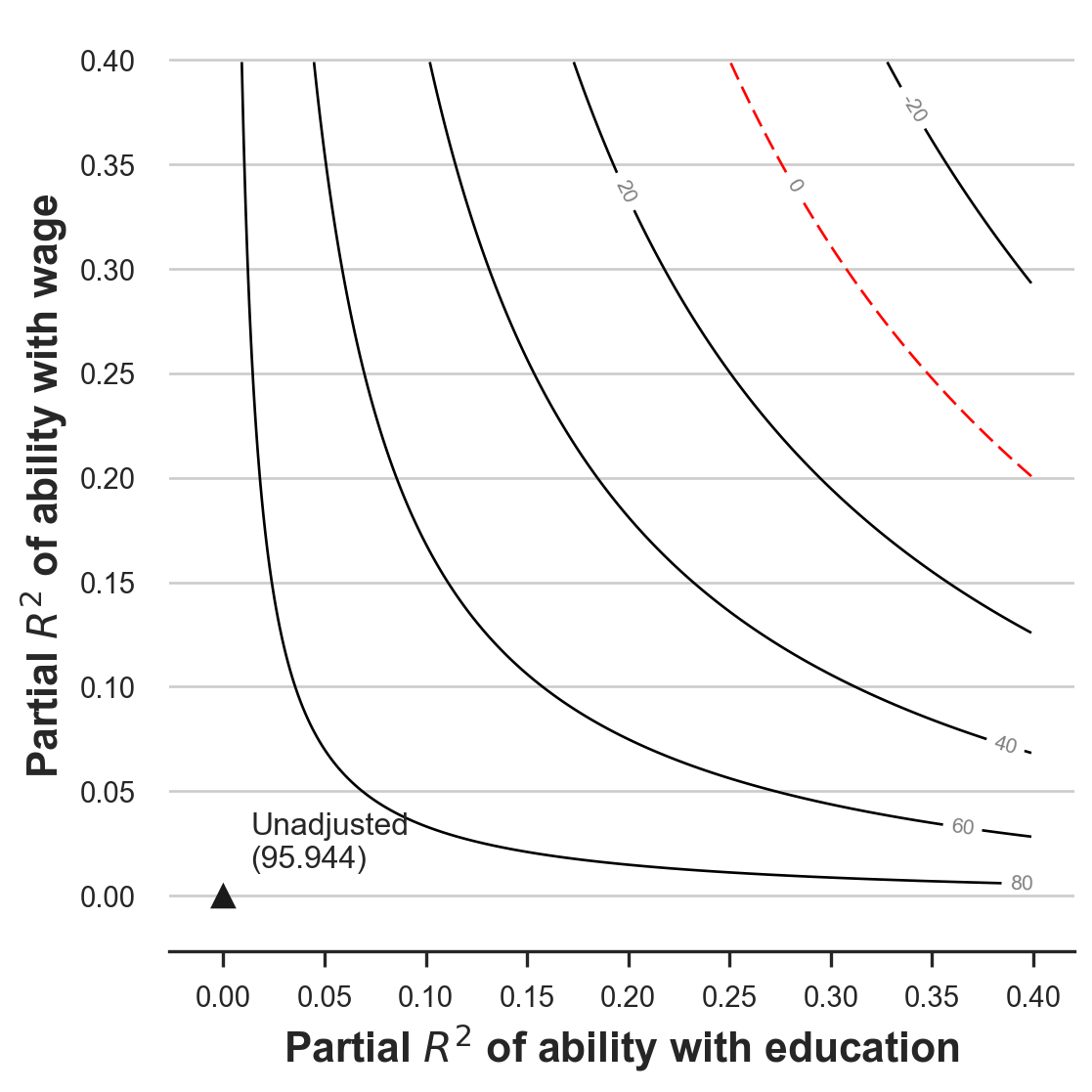
In the plot, we see how the partial (because conditional on age and gender) $R^2$ of ability with education and wage affects the estimated coefficient of education on wage. The $(0,0)$ coordinate, marked with a triangle, corresponds to the current estimate and reflects what would happen if ability had no explanatory power for both wage with education: nothing. As the explanatory power of ability grows (moving upwards and rightwards from the triangle), the estimated coefficient decreases, as marked by the level curves, until it becomes zero at the dotted red line.
How should we interpret the plot? We can see that we need ability to explain around 30% of the residual variation in both education and wage in order for the effect of education on wages to disappear, corresponding to the red line.
One question that you might (legitimately) have now is: what is 30%? Is it big or is it small? We can get a sense of the magnitude of the partial $R^2$ by benchmarking the results with the residual variance explained by another observed variable. Let’s use age for example.
The Sensemakr function accepts the following optional arguments:
benchmark_covariates: the covariate to use as a benchmarkkdandky: these arguments parameterize how many times stronger the unobserved variable (ability) is related to the treatment (kd) and to the outcome (ky) in comparison to the observed benchmark covariate (age). In our example, settingkdandkyequal to $[0.5, 1, 2]$ means we want to investigate the maximum strength of a variable half, same, or twice as strong asage(in explainingeducationandwagevariation).
sensitivity = sensemakr.Sensemakr(model = short_model,
                                  treatment = "education",
                                  benchmark_covariates = "age",
                                  kd = [0.5, 1, 2],
                                  ky = [0.5, 1, 2])
sensitivity.plot()
plt.xlabel("Partial $R^2$ of ability with education");
plt.ylabel("Partial $R^2$ of ability with wage");
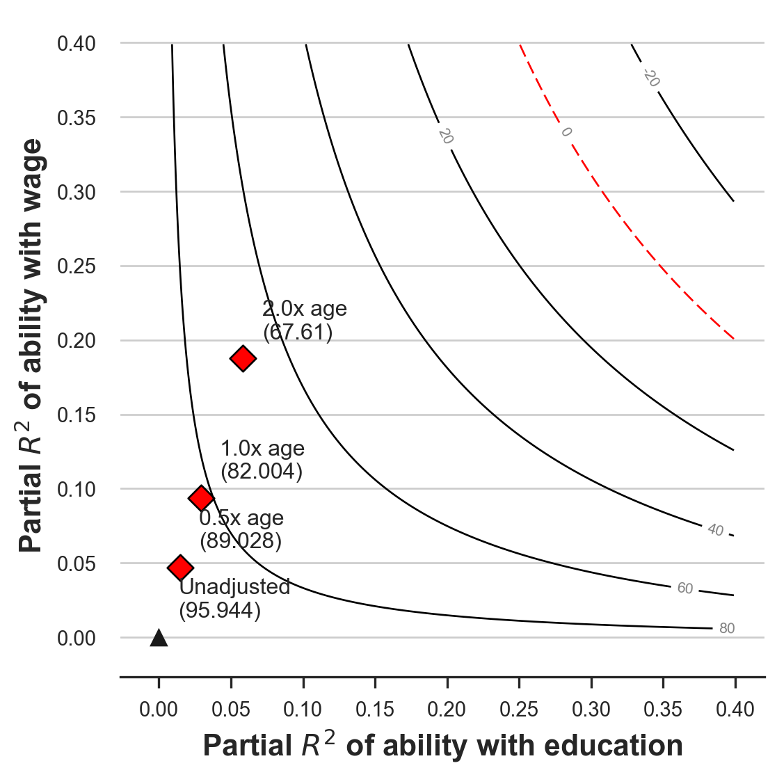
It looks like even if ability had twice as much explanatory power as age, the effect of education on wage would still be positive. But would it be statistically significant?
We can repeat the same exercise, looking at the t-statistic instead of the magnitude of the coefficient. We just need to set the sensitivity_of option in the plotting function equal to t-value.
The question that we are trying to answer in this case is:
How much of the residual variation in
education(x axis) andwage(y axis) doesabilityneed to explain in order for the effect ofeducationonwagesto become not significant?
sensitivity.plot(sensitivity_of = 't-value')
plt.xlabel("Partial $R^2$ of ability with education");
plt.ylabel("Partial $R^2$ of ability with wage");
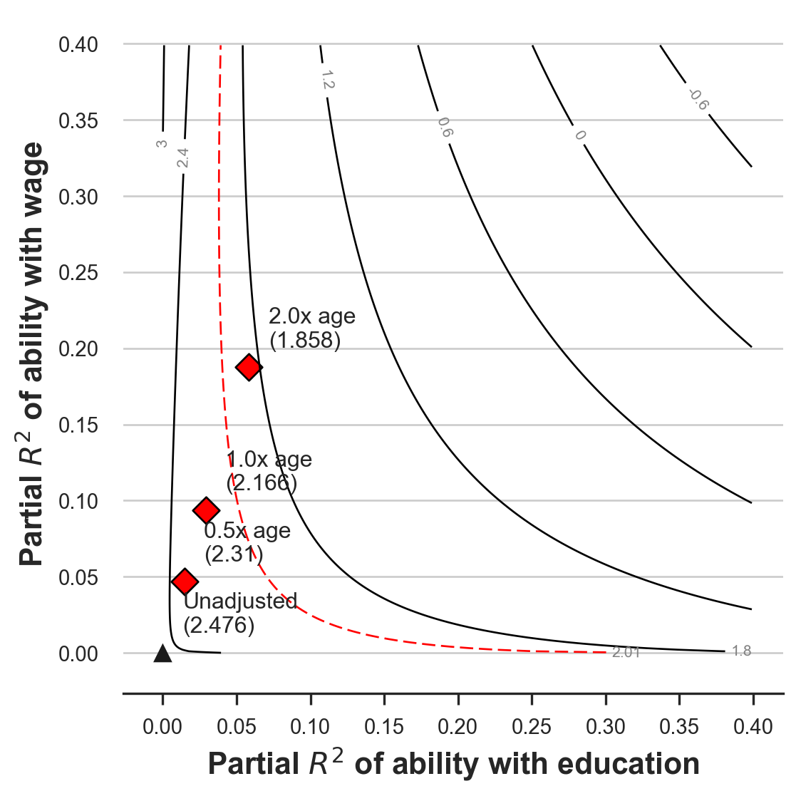
From the plot, we can see, we need ability to explain around 5% to 10% of the residual variation in both education and wage in order for the effect of education on wage not to be significant. In particular, the red line plots the level curve for the t-statistic equal to 2.01, corresponding to a 5% significance level. From the comparison with age, we see that a slightly stronger explanatory power (bigger than 1.0x age) would be sufficient to make the coefficient of education on wage not statistically significant.
Conclusion
In this post, I have introduced the concept of omitted variable bias. We have seen how it’s computed in a simple linear model and how we can exploit qualitative information about the variables to make inference in presence of omitted variable bias.
These tools are extremely useful since omitted variable bias is essentially everywhere. First of all, there are always factors that we do not observe, such as ability in our toy example. However, even if we could observe everything, omitted variable bias can also emerge in the form of model misspecification. Suppose that wages depended on age in a quadratic way. Then, omitting the quadratic term from the regression introduces bias, which can be analyzed with the same tools we have used for ability.
References
[1] C. Cinelli, C. Hazlett, Making Sense of Sensitivity: Extending Omitted Variable Bias (2019), Journal of the Royal Statistical Society.
[2] V. Chernozhukov, C. Cinelli, W. Newey, A. Sharma, V. Syrgkanis, Long Story Short: Omitted Variable Bias in Causal Machine Learning (2022), working paper.
Related Articles
Code
You can find the original Jupyter Notebook here:
https://github.com/matteocourthoud/Blog-Posts/blob/main/ovb.ipynb
I hold a PhD in economics from the University of Zurich. Now I work at the intersection of economics, data science and statistics. I regularly write about causal inference on Medium.