Comparing ATE Estimators
%matplotlib inline
%config InlineBackend.figure_format = 'retina'
from src.utils import *
from src.dgp import dgp_compare
df = dgp_compare().generate_data(include_beta=True)
df.head()
| outcome | treated | male | age | income | beta | |
|---|---|---|---|---|---|---|
| 0 | 38.68 | False | 0 | 28.0 | 1514.0 | 2.726425 |
| 1 | 37.81 | False | 1 | 47.0 | 1524.0 | 2.777192 |
| 2 | 27.70 | False | 0 | 60.0 | 2683.0 | 0.247312 |
| 3 | 29.56 | False | 0 | 29.0 | 3021.0 | 2.632797 |
| 4 | 36.83 | False | 0 | 25.0 | 1859.0 | 1.724331 |
np.mean(df['beta'])
2.0
Simple difference
smf.ols('outcome ~ treated', data=df).fit().summary().tables[1]
| coef | std err | t | P>|t| | [0.025 | 0.975] | |
|---|---|---|---|---|---|---|
| Intercept | 30.8496 | 0.091 | 340.817 | 0.000 | 30.672 | 31.027 |
| treated[T.True] | -0.0060 | 0.118 | -0.051 | 0.959 | -0.238 | 0.226 |
Regression with control
smf.ols('outcome ~ treated + male + age + income', data=df).fit().summary().tables[1]
| coef | std err | t | P>|t| | [0.025 | 0.975] | |
|---|---|---|---|---|---|---|
| Intercept | 29.5761 | 0.272 | 108.833 | 0.000 | 29.043 | 30.109 |
| treated[T.True] | 2.2682 | 0.129 | 17.623 | 0.000 | 2.016 | 2.520 |
| male | 4.8568 | 0.104 | 46.688 | 0.000 | 4.653 | 5.061 |
| age | -0.1215 | 0.006 | -21.752 | 0.000 | -0.132 | -0.111 |
| income | 0.0014 | 9e-05 | 16.032 | 0.000 | 0.001 | 0.002 |
Matching
from causalml.match import NearestNeighborMatch, create_table_one

X = ['male', 'age', 'income']
psm = NearestNeighborMatch(replace=True, ratio=1, random_state=42)
df_matched = psm.match(data=df,
                       treatment_col="treated",
                       score_cols=X)
smf.ols('outcome ~ treated', data=df_matched).fit().summary().tables[1]
| coef | std err | t | P>|t| | [0.025 | 0.975] | |
|---|---|---|---|---|---|---|
| Intercept | 29.5347 | 0.078 | 380.105 | 0.000 | 29.382 | 29.687 |
| treated[T.True] | 1.6918 | 0.110 | 15.396 | 0.000 | 1.476 | 1.907 |
IPW
df["pscore"] = smf.logit("np.rint(treated) ~ male + age + income", data=df).fit(disp=False).predict()
w = 1 / (df["pscore"] * df["treated"] + (1-df["pscore"]) * (1-df["treated"]))
smf.wls("outcome ~ treated", weights=w, data=df).fit().summary().tables[1]
| coef | std err | t | P>|t| | [0.025 | 0.975] | |
|---|---|---|---|---|---|---|
| Intercept | 30.2572 | 0.083 | 362.783 | 0.000 | 30.094 | 30.421 |
| treated[T.True] | 1.6806 | 0.116 | 14.429 | 0.000 | 1.452 | 1.909 |
R Learner
from causalml.inference.meta import BaseRLearner
from lightgbm import LGBMRegressor

BaseRLearner(learner=LGBMRegressor()).estimate_ate(X=df[X], treatment=df['treated'], y=df['outcome'])
(array([1.6529302]), array([1.65076231]), array([1.65509809]))
S Learner
from causalml.inference.meta import BaseSLearner

BaseSLearner(learner=LGBMRegressor()).estimate_ate(X=df[X], treatment=df['treated'], y=df['outcome'])
array([2.08090912])
T Learner
from causalml.inference.meta import BaseTLearner

BaseTLearner(learner=LGBMRegressor()).estimate_ate(X=df[X], treatment=df['treated'], y=df['outcome'])
(array([2.05252873]), array([1.86063479]), array([2.24442267]))
X Learner
from causalml.inference.meta import BaseXLearner

BaseXLearner(learner=LGBMRegressor()).estimate_ate(X=df[X], treatment=df['treated'], y=df['outcome'])
(array([2.0255193]), array([1.83456903]), array([2.21646956]))
DR Learner
from causalml.inference.meta import BaseDRLearner

BaseDRLearner(learner=LGBMRegressor()).estimate_ate(X=df[X], treatment=df['treated'], y=df['outcome'])
(array([2.08923293]), array([1.8921804]), array([2.28628547]))
Compare All
def simulate(dgp, K=100):

    # Initialize coefficients
    results = pd.DataFrame(columns=['k', 'Estimator', 'Estimate'])
    names = ['1. Diff ', '2. Reg  ', '3. Match', '4. IPW  ',
             '5. R lrn', '6. S lrn', '7. T lrn', '8. X lrn', '9. DRlrn']

    # Compute coefficients
    for k in range(K):
        print(f"Simulation {k}/{K}", end="\r")
        temp = pd.DataFrame({'k': [k] * len(names),
                             'Estimator': names,
                             'Estimate': [0] * len(names)})

        # Draw data
        df = dgp.generate_data(seed=k)

        # Single diff
        temp['Estimate'][0] = smf.ols('outcome ~ treated', data=df).fit().params[1]

        # Regression with controls
        temp['Estimate'][1] = smf.ols(f'outcome ~ treated + male + age + income', data=df).fit().params[1]

        # Matching
        psm = NearestNeighborMatch(replace=True, ratio=1)
        df_matched = psm.match(data=df, treatment_col="treated", score_cols=X)
        temp['Estimate'][2] = smf.ols('outcome ~ treated', data=df_matched).fit().params[1]

        # IPW
        df["pscore"] = smf.logit("np.rint(treated) ~ male + age + income", data=df).fit(disp=False).predict()
        w = 1 / (df["pscore"] * df["treated"] + (1-df["pscore"]) * (1-df["treated"]))
        temp['Estimate'][3] = smf.wls("outcome ~ treated", weights=w, data=df).fit().params[1]

        # R Learner
        temp['Estimate'][4] = BaseRLearner(learner=LGBMRegressor()).estimate_ate(X=df[X], treatment=df['treated'], y=df['outcome'])[0][0]

        # S Learner
        temp['Estimate'][5] = BaseSLearner(learner=LGBMRegressor()).estimate_ate(X=df[X], treatment=df['treated'], y=df['outcome'])[0]

        # T Learner
        temp['Estimate'][6] = BaseTLearner(learner=LGBMRegressor()).estimate_ate(X=df[X], treatment=df['treated'], y=df['outcome'])[0][0]

        # X Learner
        temp['Estimate'][7] = BaseXLearner(learner=LGBMRegressor()).estimate_ate(X=df[X], treatment=df['treated'], y=df['outcome'])[0][0]

        # DR Learner
        temp['Estimate'][8] = BaseDRLearner(learner=LGBMRegressor()).estimate_ate(X=df[X], treatment=df['treated'], y=df['outcome'])[0][0]

        # Combine estimates
        results = pd.concat((results, temp))

    return results.reset_index(drop=True)
results = simulate(dgp=dgp_compare())
Simulation 99/100
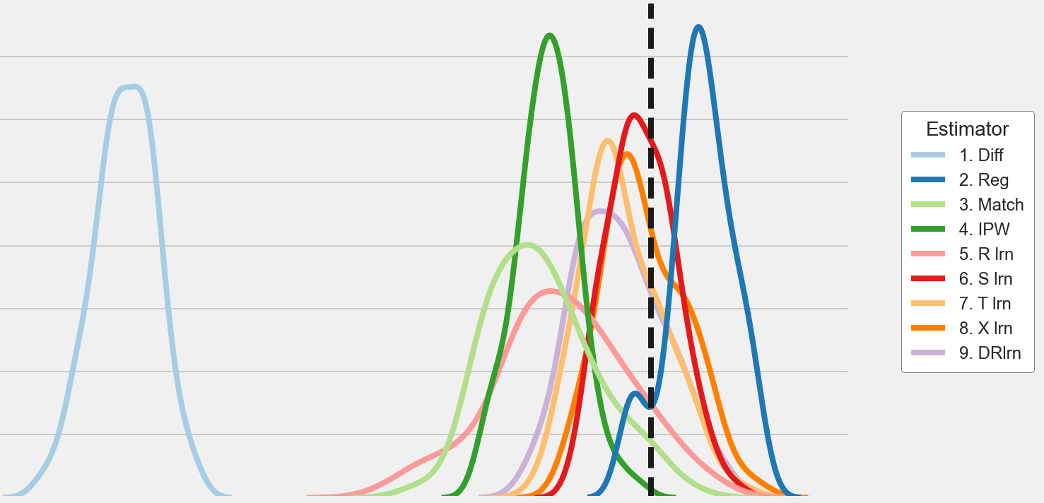
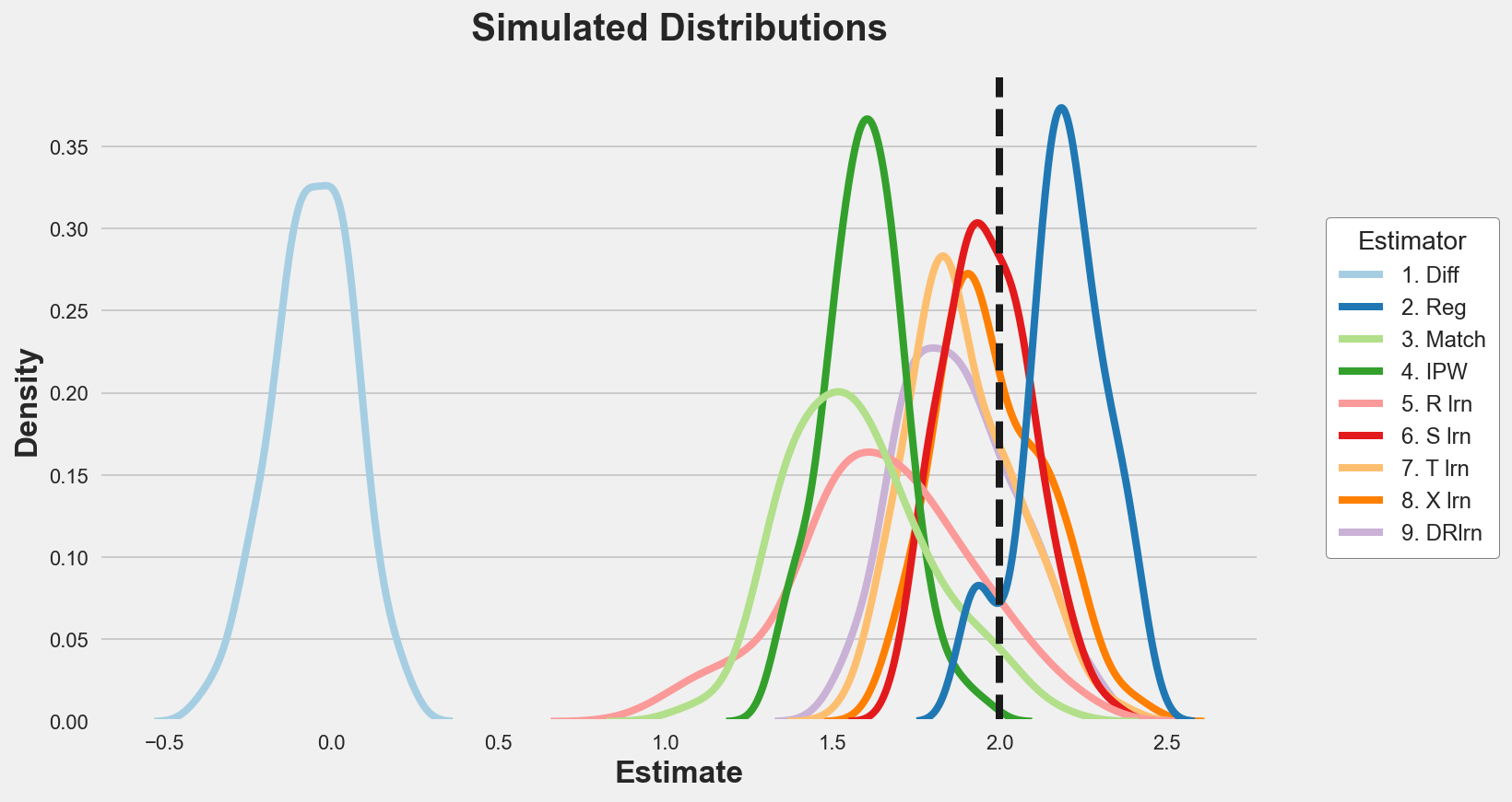
Let’s plot the distribution of the estimated parameters.
p = sns.kdeplot(data=results, x="Estimate", hue="Estimator", legend=True);
sns.move_legend(p, "upper left", bbox_to_anchor=(1.05, 0.8))
plt.axvline(x=2, c='k', ls='--');
plt.title('Simulated Distributions');
We can also tabulate the simulated mean and standard deviation of each estimator.
results.groupby('Estimator').agg(mean=("Estimate", "mean"), std=("Estimate", "std"))
| mean | std | |
|---|---|---|
| Estimator | ||
| 1. Diff | -0.054010 | 0.120718 |
| 2. Reg | 2.190934 | 0.126232 |
| 3. Match | 1.575239 | 0.211772 |
| 4. IPW | 1.596031 | 0.119129 |
| 5. R lrn | 1.649703 | 0.263321 |
| 6. S lrn | 1.963797 | 0.129638 |
| 7. T lrn | 1.891307 | 0.160480 |
| 8. X lrn | 1.975699 | 0.161004 |
| 9. DRlrn | 1.876465 | 0.173318 |
The only unbiased estimators seems to be the S-learner and the X-learner, followed by T-learner, DR-learner and linear regression.
he S-learner however is more efficient.
I hold a PhD in economics from the University of Zurich. Now I work at the intersection of economics, data science and statistics. I regularly write about causal inference on Medium.